In preparation for an upcoming 1300 aggregate Palma match to be fired at 800, 900, and 1000 yards over two days, I have measured the volume of 200 Winchester 223 cases that are otherwise ready to shoot. These cases have a mean as well as median capacity of 30.4 in grains of H2O (from here forward I will refer to grains of H2O as simply “grains”). The standard deviation was 0.12 grains, with a minimum of 30.13 and maximum of 30.88. With the expectation of 20 to 35 fps muzzle velocity per grain variation in case capacity, I expected the velocity variation to be between roughly 15 and 25 fps between the cases near the min and those near the max.
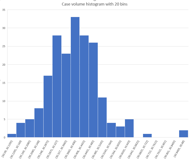
Ordering the cases from low to high volume gives the following distribution:

The majority of cases are between 30.2 and 30.55 grains with tails beyond those thresholds. I removed all these cases in the tails from the batch that I will be shooting at the upcoming match.
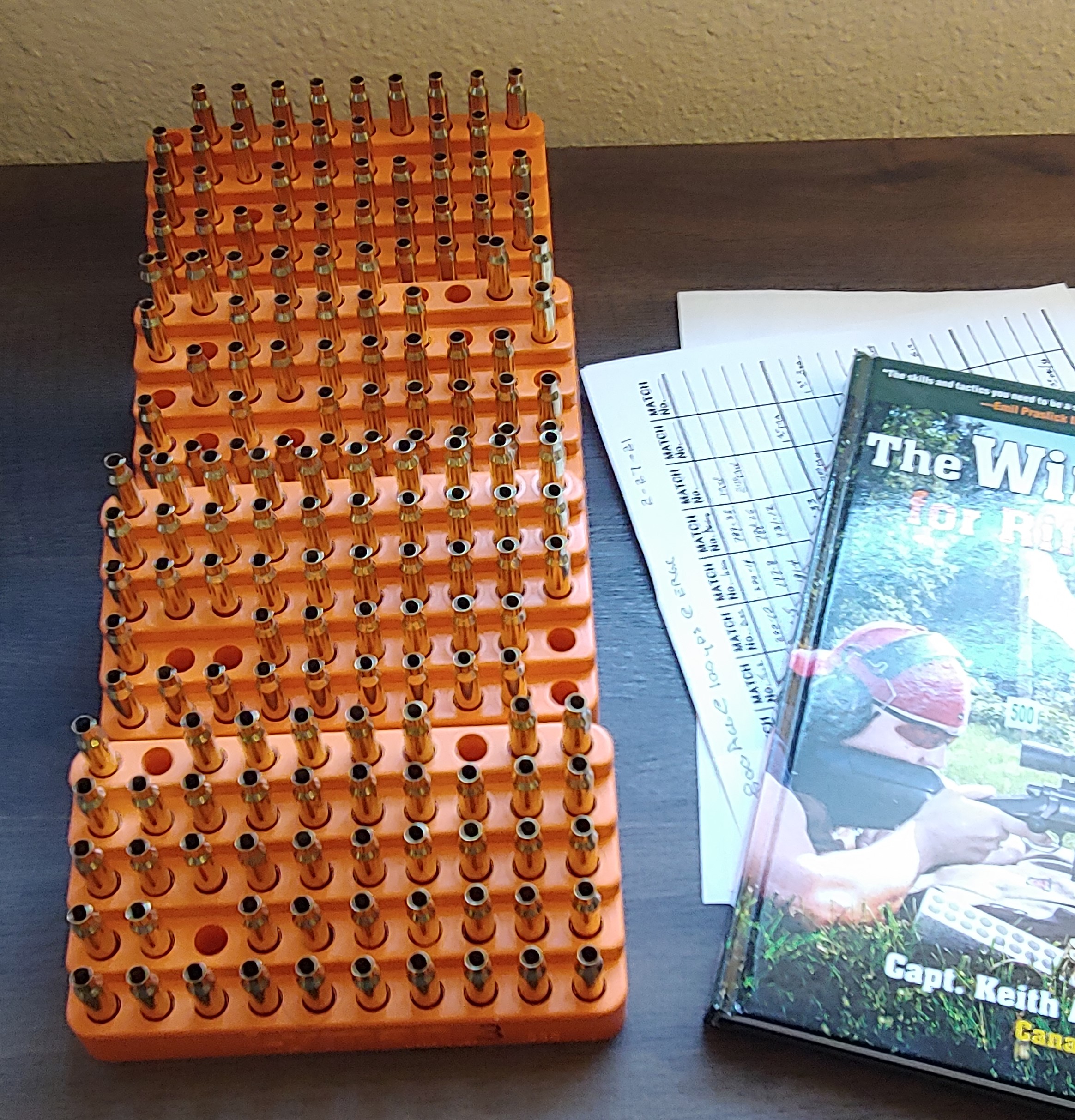
These rounds will be loaded with Hornady 90 grain A-Tip bullets to an OAL of approximately 2.45 inches. I expect to reach approximately 2600 fps with this ammunition at the muzzle.
For this study, I took the high and low six cases at each end of the distribution to measure velocity for comparison. My plan is two-fold, two see if these outliers (using this term loosely) can significantly effect my scores at 600 to 1000 yards, and if so, by how much. This is a small sample size as I want to keep the cases that are not at the tail ends of the distribution for the upcoming competition.
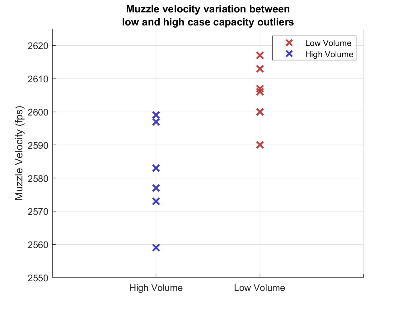
After shooting the 12 rounds I found that the muzzle velocity of the high-volume cases was 2581 fps with SD of 9.7 fps and the muzzle velocity of the low-volume cases was 2606 fps with SD of 14.9 fps. This gives a total spread of 25 fps, at the high end of the expected range.
Notice how the high capacity cases have LOWER velocity than the low capacity cases. This reflects the higher pressure generated by equal powder charge weights in a smaller volume, and is in agreement qualitatively with Quickload as well as general experience.
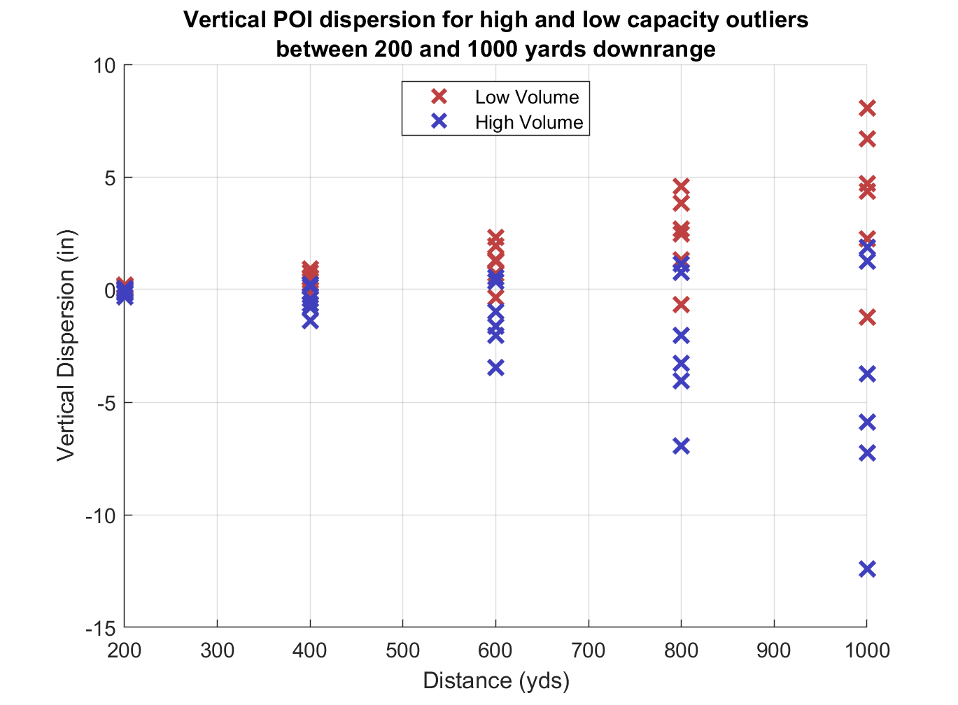
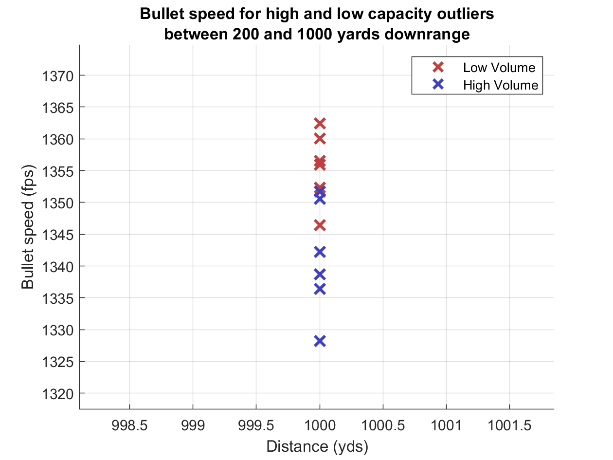
Running this data through a custom ballistics calculator that uses the mean velocity to get a fixed launch angle for all rounds gives the following vertical variation at the target for distances between 200 and 1000 yards:
Will this humble 223 load be capable of 1000 yard performance? Here’s how the bullet speed drops with distance for this load using Hornady’s G1 BC of 0.585.
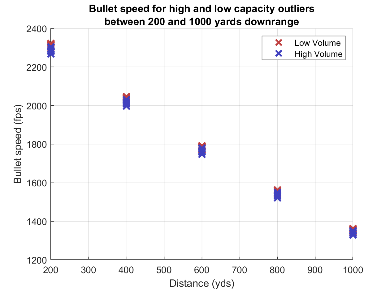
Taking the rule of thumb for the transonic limit of 1.2 Mach, in which we select a Mach 1 value of 1125 fps corresponding to air at 68 degrees F which gives a transonic limit of 1350 fps. Our ammunition comes out right at the limit, and its performance has been proven in competition as well.
In my experience a bullet need not be going too fast at the target to perform with good accuracy. Provided the bullet is properly stabilized it will continue to exhibit good accuracy to Mach 1.1 and potentially lower. It is running out of gas for sure at Mach 1.2 though so that is a good speed to aim for at the target.
So what does this all really mean for a competitive target shooter or anyone else who wants to place rounds accurately at long range? Let’s start at the low end of long range, 600 yards, usually referred to as mid-range by high power competitors. Here is where the rubber hits the road.
Suppose a sling shooter and his weapon are able, all things being equal, to hold the 10 ring most of the time at 600 yards and 1000 yards. We can simulate such a shooter, who would have a mean radius right around 0.9 (see ballistipedia.com for a proper explanation of mean radius). We can also neglect wind for this study but add in the vertical variation due to variation in muzzle velocity. At 600 yards, how many points and X’s would this shooter give up due to high or low capacity cases? Let’s have a look at the extreme example in which the shooter only shoots the cases at the tails of the distribution. Simulating 10 different groups at 600 yards we would have the perfect cases on the left and the tail-capacity cases on the right.
Note: the inner circle is the F-Class X ring. Clearly these are not F-Class groups being simulated and I will address the effect of muzzle velocity in competitive F-Class in an upcoming post.
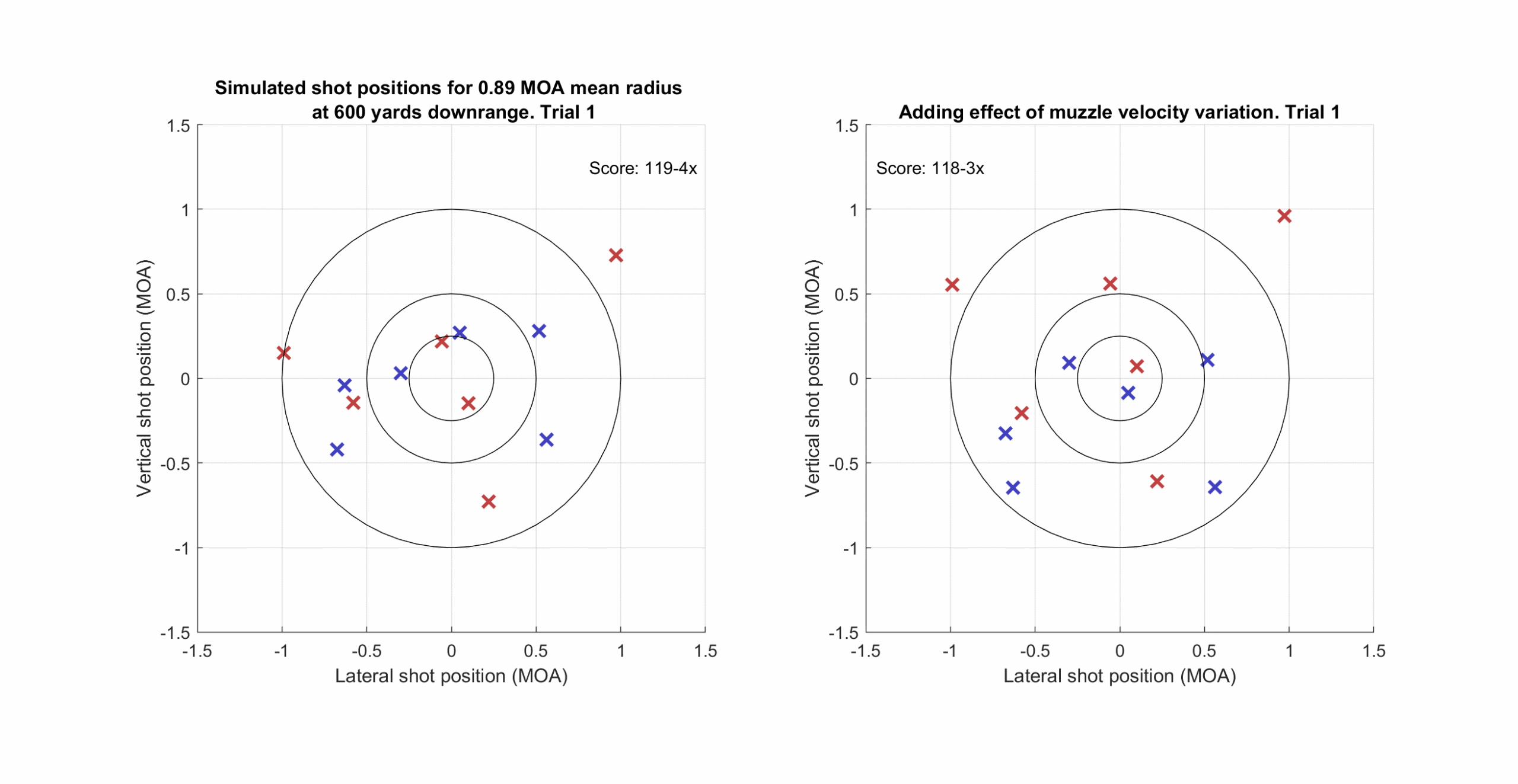
We see our shooter dropping a couple points and X’s due to case capacity variation most of the time. But we know that most of our cases are going to be in the good portion of the distribution, not at the tail. So an outlier could cost us a point, but we see why top shooters who do not measure and account for case volume rarely drop points and keep on winning anyway. Thank goodness that shooting, especially from a sling, still comes down to shooting ability, especially the general fundamentals and wind reading. But still, a competitive match could still come down to one or two rounds with relatively high or low muzzle velocity.
At 1000 yards the situation is a little bit more dramatic, but still we’re talking a few points or X’s and this for all cases at extreme ends of the distribution:
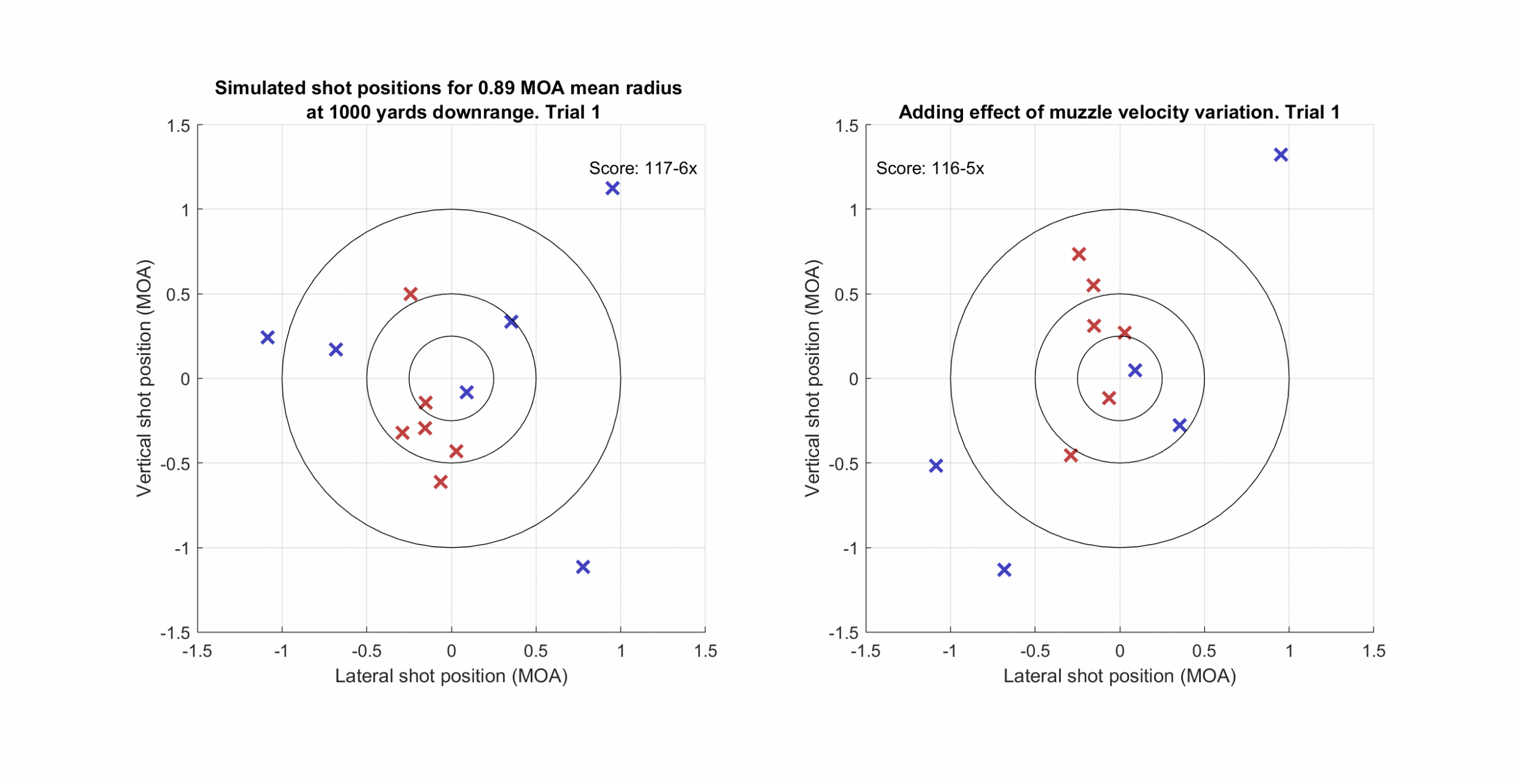
I find it amusing that sometimes inaccuracy in the weapon and ammunition can work to our favor. If we throw a shot high that would otherwise have been low due to other random variation in the weapon, wind, and ammunition, then we get lucky and save a point or two. But in the aggregate we cannot achieve winning scores consistently in this way.
So we see that muzzle velocity variation due to case capacity variation is another knob we can turn in our pursuit of perfection, but we still have to be good at shooting to reach our full potential and win matches.